CS-466/566: Math for AI

Module 04: Eigenvalues and Eigenvectors

Dr. Mahmoud Mahmoud

The University of Alabama

2026-03-23

1. Eigenproblems Intuition●

2. Mathematical Properties○

3. Diagonalization○

4. Application: Google PageRank○

Eigenvectors & Eigenvalues: Intuition

Eigenvector Animation

Eigenvectors & Eigenvalues: Definition

Eigenvalue Equation:

\[A\mathbf{x} = \lambda \mathbf{x}\]

What it means:

Eigenvector $\mathbf{x}$: Direction unchanged by transformation
Eigenvalue $\lambda$: Scaling factor applied to that direction
What it means: Some directions are “special” - they don’t get rotated!

1. Eigenproblems Intuition✓

2. Mathematical Properties●

3. Diagonalization○

4. Application: Google PageRank○

Mathematical Properties

Start with: $A\mathbf{x} = \lambda \mathbf{x}$

Attempt to solve for $\mathbf{x}$: \[A\mathbf{x} - \lambda \mathbf{x} = \mathbf{0}\] \[ (A - \lambda)\mathbf{x} = \mathbf{0} \quad \text{$\small❌$ (Matrix − Number is illegal)} \]

Correct way: Multiply $\lambda$ by Identity $I$: \[A\mathbf{x} - \lambda I \mathbf{x} = \mathbf{0}\] \[(A - \lambda I)\mathbf{x} = \mathbf{0} \quad {\small \text{✅ (Matrix - Matrix)}}\]

Steps to Find Eigenvalues & Eigenvectors

Step 1: Build characteristic polynomial \[\det(A - \lambda I) = 0\]

Step 2: Solve for eigenvalues $\lambda_i$

Step 3: For each $\lambda_i$, solve \[(A - \lambda_i I)\mathbf{x} = \mathbf{0}\]

Step 4: Find basis for nullspace = eigenvectors

Example (1/5): Characteristic Equation

Matrix: \[A = \begin{bmatrix}2 & 1\\1 & 2\end{bmatrix}\]

Step 1: Setup Characteristic Equation \[ A - \lambda I = \begin{bmatrix}2 & 1\\1 & 2\end{bmatrix} - \begin{bmatrix}\lambda & 0\\0 & \lambda\end{bmatrix} = \begin{bmatrix}2-\lambda & 1\\1 & 2-\lambda\end{bmatrix} \]

Step 2: Compute Determinant \[ \det(A - \lambda I) = (2-\lambda)(2-\lambda) - (1)(1) \]

Example (2/5): Solving for Eigenvalues

Step 2 (Continued): Simplify \[ \det(A - \lambda I) = (4 - 4\lambda + \lambda^2) - 1 \] \[ = \lambda^2 - 4\lambda + 3 \]

Step 3: Solve $\lambda^2 - 4\lambda + 3 = 0$ \[ (\lambda - 3)(\lambda - 1) = 0 \] \[ \lambda_1 = 3, \quad \lambda_2 = 1 \]

Example (3/5): Eigenvectors ($\lambda_1 = 3$)

Solve $(A - 3I)\mathbf{x} = \mathbf{0}$

\[ \left[\begin{array}{cc|c} 2-3 & 1 & 0 \\ 1 & 2-3 & 0 \end{array}\right] \Rightarrow \left[\begin{array}{cc|c} -1 & 1 & 0 \\ 1 & -1 & 0 \end{array}\right] \]

System of Equations: \[ -x + y = 0 \Rightarrow x = y \]

Pick a value: Let $x=1$, then $y=1$. Eigenvector: $\mathbf{x}_1 = \begin{bmatrix} 1 \\ 1 \end{bmatrix}$

Example (4/5): Eigenvectors ($\lambda_2 = 1$)

Solve $(A - 1I)\mathbf{x} = \mathbf{0}$

\[ \left[\begin{array}{cc|c} 2-1 & 1 & 0 \\ 1 & 2-1 & 0 \end{array}\right] \Rightarrow \left[\begin{array}{cc|c} 1 & 1 & 0 \\ 1 & 1 & 0 \end{array}\right] \]

System of Equations: \[ x + y = 0 \Rightarrow x = -y \]

Pick a value: Let $y=1$, then $x=-1$. Eigenvector: $\mathbf{x}_2 = \begin{bmatrix} -1 \\ 1 \end{bmatrix}$

Example (5/5): Summary Results

Matrix: \[A = \begin{bmatrix}2 & 1\\1 & 2\end{bmatrix}\]

Eigenvalue-Eigenvector Pairs:

Pair 1: \[ \lambda_1 = 3 \] \[ \mathbf{x}_1 = \begin{bmatrix}1\\1\end{bmatrix} \]

Pair 2: \[ \lambda_2 = 1 \] \[ \mathbf{x}_2 = \begin{bmatrix}-1\\1\end{bmatrix} \]

Computing in NumPy: `eig()`

import numpy as np

#> Our 2x2 Matrix from the example
A = np.array([[2, 1], [1, 2]])

#> Compute eigenvalues and eigenvectors
lambdas, vectors = np.linalg.eig(A)

print(f"Eigenvalues: {lambdas}")
print(f"Eigenvectors:\n{vectors}")

Eigenvalues: [3. 1.]
Eigenvectors:
[[ 0.70710678 -0.70710678]
 [ 0.70710678  0.70710678]]

Note: The eigenvectors are normalized (length = 1).

Pattern Discovery

Look at our results from the previous example: \[ \lambda_1 = 3, \quad \lambda_2 = 1 \] \[ \text{Sum} = 4, \quad \text{Product} = 3 \]

Look at the original matrix: \[ A = \begin{bmatrix}2 & 1\\1 & 2\end{bmatrix} \] \[ \text{Trace (sum of diagonal)} = 2 + 2 = 4 \] \[ \text{Determinant} = (2)(2) - (1)(1) = 3 \]

Coincidence? I think not! 🤔

Mathematical Properties

Algebraic Definition

Characteristic Equation: Values $\lambda$ where matrix becomes singular $\det(A - \lambda I) = 0$
Null Space: Vectors $\mathbf{x}$ in the null space of shift $(A - \lambda I)\mathbf{x} = \mathbf{0}$

Verify Your Results

Sum Rule (Trace): Sum of diagonal = Sum of eigenvalues \[ \text{tr}(A) = \sum \lambda_i \]
Product Rule (Determinant): Determinant = Product of eigenvalues \[ \det(A) = \prod \lambda_i \]

Your Turn: Quick Check

Matrix: \[ B = \begin{bmatrix} 3 & 1 \\ 1 & 3 \end{bmatrix} \]

Task: Find the eigenvalues without solving the characteristic polynomial!

Trace: $3 + 3 = 6$ \[ \Rightarrow \lambda_1 + \lambda_2 = 6 \]

Determinant: $9 - 1 = 8$ \[ \Rightarrow \lambda_1 \cdot \lambda_2 = 8 \]

Find two numbers that sum to 6 and multiply to 8: \[ \lambda_1 = 4, \quad \lambda_2 = 2 \]

1. Eigenproblems Intuition✓

2. Mathematical Properties✓

3. Diagonalization●

4. Application: Google PageRank○

The Matrix of Eigenvectors

Collect all eigenvectors into one matrix $C$

\[ C = \begin{bmatrix} | & | & & | \\ \mathbf{x}_1 & \mathbf{x}_2 & \cdots & \mathbf{x}_n \\ | & | & & | \end{bmatrix} \]

And eigenvalues into a diagonal matrix $D$

\[ D = \begin{bmatrix} \lambda_1 & 0 & \cdots & 0 \\ 0 & \lambda_2 & \cdots & 0 \\ \vdots & \vdots & \ddots & \vdots \\ 0 & 0 & \cdots & \lambda_n \end{bmatrix} \]

Key Relationship

\[ AC = CD \implies A = CDC^{-1} \]

Matrix Exponentiation

Question: How to compute $A^k$ efficiently for $n \times n$ matrix? (Naive: $O(kn^3)$)

Lets transform a vector $\mathbf{x}$ by $A$ for $k$ times: \[ A^k \mathbf{x} \]

Better Way for Matrix Exponentiation

Proof Strategy: Check what happens to $A^k$

\[ A^k = \underbrace{A \cdot A \cdot A \cdots A}_{k \text{ times}} \]

Substitute $A = CDC^{-1}$:

\[ A^k = (CDC^{-1}) (CDC^{-1}) (CDC^{-1}) \cdots (CDC^{-1}) \]

Cancel Internal Terms:

\[ A^k = C D (\underbrace{C^{-1}C}_{I}) D (\underbrace{C^{-1}C}_{I}) D \cdots (\underbrace{C^{-1}C}_{I}) D C^{-1} \]

Result (Powers of Diagonal Matrix): \[ A^k = C D^k C^{-1} \]

Conclusion: $A^k$ scales eigenvectors by $\lambda^k$

1. Eigenproblems Intuition✓

2. Mathematical Properties✓

3. Diagonalization✓

4. Application: Google PageRank●

The “Billion Dollar” Eigenvector

The Question How does Google search rank billions of webpages?

The Intuition - A page is “important” if important pages link to it. - It’s a popularity contest… but weighted!

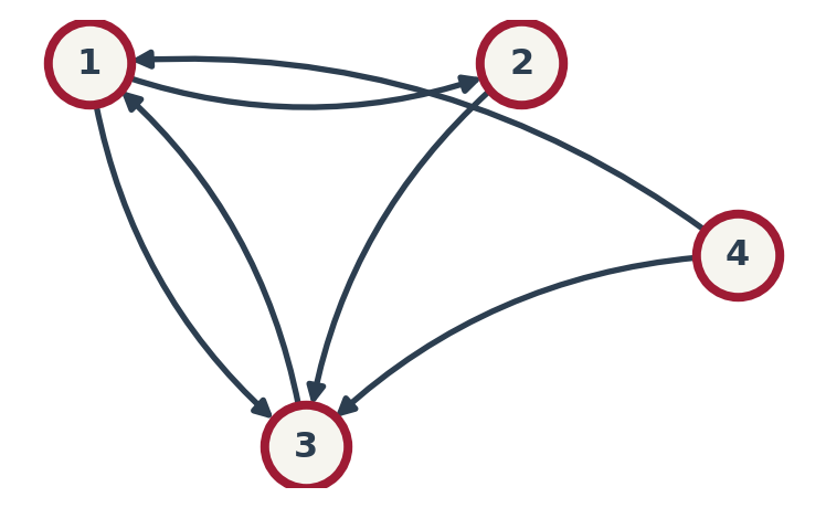
The Web as a Matrix

Rule: If Page $j$ links to Page $i$, it “votes” for $i$. $M_{ij} = P(j \to i)$.

How to build Column $j$ (Page $j$):

Count outgoing links $k$.
Put $1/k$ in rows of target pages.

Example:

Col 1 (Page 1): Links to {2, 3} ($k=2$). $\Rightarrow$ Rows 2 & 3 get $1/2$.
Col 3 (Page 3): Links to {1} ($k=1$). $\Rightarrow$ Row 1 gets $1/1 = 1$.

Example Matrix $A$: \[ A = \begin{bmatrix} 0 & 0 & 1 & 1/2 \\ 1/2 & 0 & 0 & 0 \\ 1/2 & 1 & 0 & 1/2 \\ 0 & 0 & 0 & 0 \end{bmatrix} \]

The Eigenvector Connection

Let $r$ be the rank vector. The rank of page $i$ is the weighted sum of ranks pointing to it.

Example for Page 3: \[ r_3 = \frac{1}{2}r_1 + 1 \cdot r_2 + \frac{1}{2}r_4 \]
(Matches Row 3 of $A$: $[1/2, 1, 0, 1/2]$)

This applies to all pages simultaneously: \[ \begin{bmatrix} r_1 \\ r_2 \\ r_3 \\ r_4 \end{bmatrix} = \begin{bmatrix} 0 & 0 & 1 & 1/2 \\ 1/2 & 0 & 0 & 0 \\ 1/2 & 1 & 0 & 1/2 \\ 0 & 0 & 0 & 0 \end{bmatrix} \begin{bmatrix} r_1 \\ r_2 \\ r_3 \\ r_4 \end{bmatrix} \] $\implies \mathbf{r} = A \mathbf{r}$

Look familiar? \[ A \mathbf{r} = 1 \cdot \mathbf{r} \] PageRank is finding the eigenvector for $\lambda = 1$!

How to Compute it?

We need to solve $A\mathbf{r} = \mathbf{r}$ for billions of pages.

The Naive Way Gaussian Elimination ($O(n^3)$)

For $n = 10^9$, this takes forever.

The Efficient Way Power Iteration:

Start with random $\mathbf{r}_0$.
$\mathbf{r}_{k+1} = A \mathbf{r}_k$.
Repeat until convergence.

Why it works? Recall: $A^k$ scales eigenvectors by $\lambda^k$. Expand $\mathbf{r}_0$ as sum of eigenvectors: $\mathbf{r}_0 = c_1 \mathbf{v}_1 + c_2 \mathbf{v}_2 + \dots$ \[ A^k \mathbf{r}_0 = c_1 (1)^k \mathbf{v}_1 + c_2 (\underbrace{\lambda_2}_{<1})^k \mathbf{v}_2 + \dots \] As $k \to \infty$, the small eigenvalues die ($0.5^{100} \approx 0$). Only $\mathbf{v}_1$ remains!

PageRank in NumPy: Defining the Matrix

import numpy as np

#> Define the Column-Stochastic Matrix A
A = np.array([
    [0,   0, 1,   0.5],
    [0.5, 0, 0,   0  ],
    [0.5, 1, 0,   0.5],
    [0,   0, 0,   0  ]
])

#> Initial Rank Vector (everyone starts equal)
r0 = np.array([0.25, 0.25, 0.25, 0.25])

Note: We use np.array to store $A$. For real web graphs, we would use scipy.sparse to save memory!

PageRank in NumPy: Eigen-Solution

#> Compute eigenvalues and eigenvectors
lambdas, vectors = np.linalg.eig(A)
print(f"Eigenvalues: {lambdas}")

#> Find the index of the eigenvalue nearest to 1.0
idx = np.where(np.isclose(lambdas, 1.0, atol=1e-8))[0][0]
rank_vector = vectors[:, idx].real

#> Normalize (so values sum to 1)
rank_vector = rank_vector / np.sum(rank_vector)

print(f"PageRank: {rank_vector}")

Eigenvalues: [ 1. +0.j  -0.5+0.5j -0.5-0.5j  0. +0.j ]
PageRank: [ 0.4  0.2  0.4 -0. ]

Insight: This is the “Exact” solution. It’s fast for small matrices but $O(n^3)$ for large ones.

PageRank in NumPy: Power Iteration

#> Iterative multiplication
r0 = np.array([0.25, 0.25, 0.25, 0.25])
r_k = r0
for i in range(20):
    r_k = A @ r_k

print(f"Iterative Result: {r_k}")

Iterative Result: [0.40014648 0.1998291  0.40002441 0.        ]

Efficiency: This only requires Matrix-Vector multiplication ($O(\text{Links})$), which is why Google can scale it to billions of pages!

CS-466/566: Math for AI

TABLE OF CONTENTS

Eigenvectors & Eigenvalues: Intuition

Eigenvectors & Eigenvalues: Definition

TABLE OF CONTENTS

Mathematical Properties

Steps to Find Eigenvalues & Eigenvectors

Example (1/5): Characteristic Equation

Example (2/5): Solving for Eigenvalues

Example (3/5): Eigenvectors (\(\lambda_1 = 3\))

Example (4/5): Eigenvectors (\(\lambda_2 = 1\))

Example (5/5): Summary Results

Computing in NumPy: `eig()`

Pattern Discovery

Mathematical Properties

Your Turn: Quick Check

TABLE OF CONTENTS

The Matrix of Eigenvectors

Matrix Exponentiation

Better Way for Matrix Exponentiation

TABLE OF CONTENTS

The “Billion Dollar” Eigenvector

The Web as a Matrix

The Eigenvector Connection

How to Compute it?

PageRank in NumPy: Defining the Matrix

PageRank in NumPy: Eigen-Solution

PageRank in NumPy: Power Iteration

Thank You!

CS-466/566: Math for AI

TABLE OF CONTENTS

Eigenvectors & Eigenvalues: Intuition

Eigenvectors & Eigenvalues: Definition

TABLE OF CONTENTS

Mathematical Properties

Steps to Find Eigenvalues & Eigenvectors

Example (1/5): Characteristic Equation

Example (2/5): Solving for Eigenvalues

Example (3/5): Eigenvectors (\(\lambda_1 = 3\))

Example (4/5): Eigenvectors (\(\lambda_2 = 1\))

Example (5/5): Summary Results

Computing in NumPy: eig()

Pattern Discovery

Mathematical Properties

Your Turn: Quick Check

TABLE OF CONTENTS

The Matrix of Eigenvectors

Matrix Exponentiation

Better Way for Matrix Exponentiation

TABLE OF CONTENTS

The “Billion Dollar” Eigenvector

The Web as a Matrix

The Eigenvector Connection

How to Compute it?

PageRank in NumPy: Defining the Matrix

PageRank in NumPy: Eigen-Solution

PageRank in NumPy: Power Iteration

Thank You!

Computing in NumPy: `eig()`